ACF
The autocorrelation function (ACF) is a measure of how random or periodic a surface is. ACF is found by creating a duplicate ((Z(x-Dx,y-Dy))) of the measured surface ((Z (x, y)), then shifting the duplicate relative to the original, in all directions. With each move the two datasets are multiplied together, and the result is integrated then normalized to the value found for zero shift, to yield a measure of the degree of overlap between the two functions. If the shifted version of the surface is identical to the original surface then the ACF is 1.00. If the shifted surface is such that all peaks align with corresponding valleys then the ACF will approach –1.00.
Values for ACF range from 1.0 (correlated) to -1.0 (uncorrelated). For a perfectly flat, infinitely large surface the ACF will stay at 1.00, as the pixels of the duplicate and original surfaces will always be identical, no matter how far the two surfaces are shifted. For a random surface, the ACF will dampen to 0 quickly as individual pixels will be as likely to align as to not.
An Example of ACF in Two Dimensions
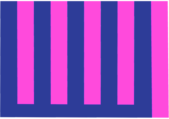
Consider the comb shown below as an example:
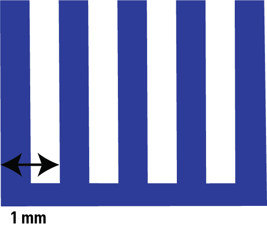
To plot the ACF we start by making a copy of the comb and aligning it directly behind the original. In this position all of the teeth perfectly overlap, and the ACF is 1.00.
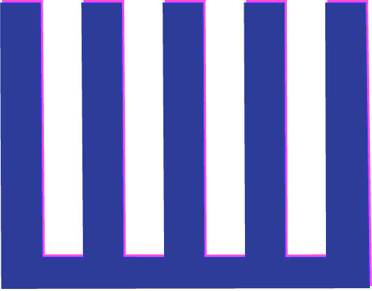
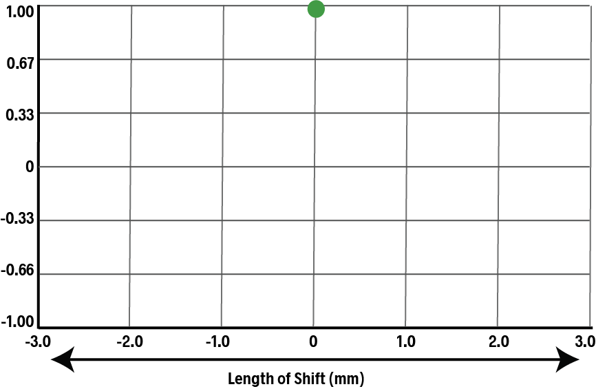
Now, we shift the duplicate comb (shown in pink) slightly to the right. The teeth now align slightly less well, and the ACF drops.
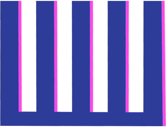
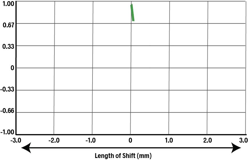
As we continue to shift the duplicate, the ACF will continue to drop with each move.

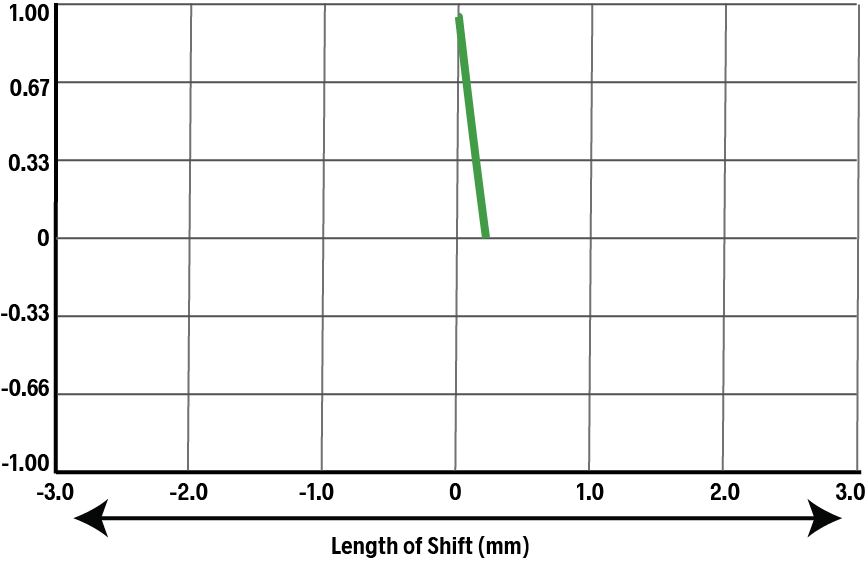
When the teeth of the duplicate overlap with the spaces of the original, the ACF will near -1.0.
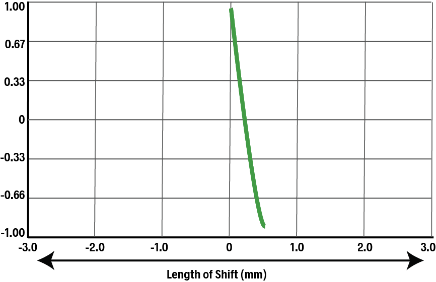
The ACF will then rise again until the duplicate is exactly one tooth spacing away from the original:

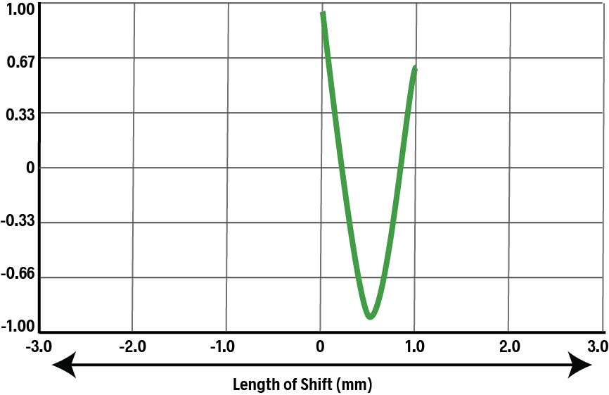
The pattern repeats as the duplicate moves farther and farther to the right:

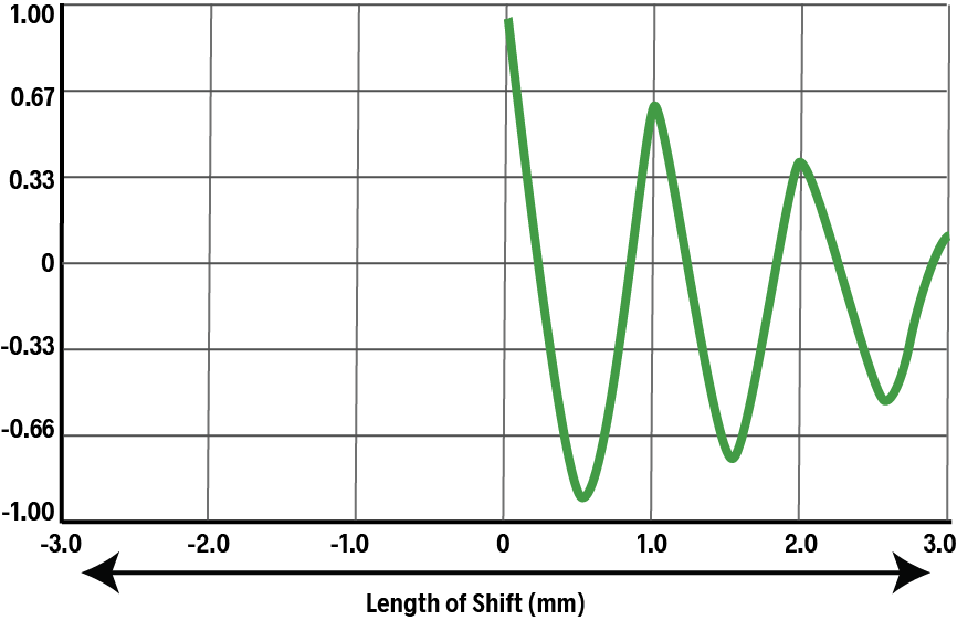
Note that the ACF tapers off as we shift the duplicate farther and farther. This is because more of the duplicate extends past any of the teeth of the original. The non-overlapping areas have 0 correlation, and thus the overall correlation drops.
Up until now we have only moved the duplicate to the right. We can also go back to the origin and then shift it to the left, which would produce an identical curve in the opposite direction:

An Example of ACF in Three Dimensions
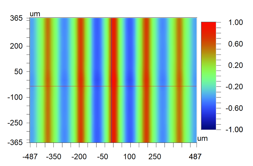
This 3D measurement of turned texture is similar to the comb example above.
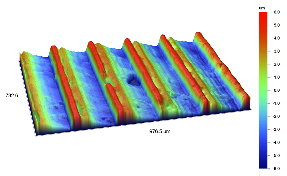
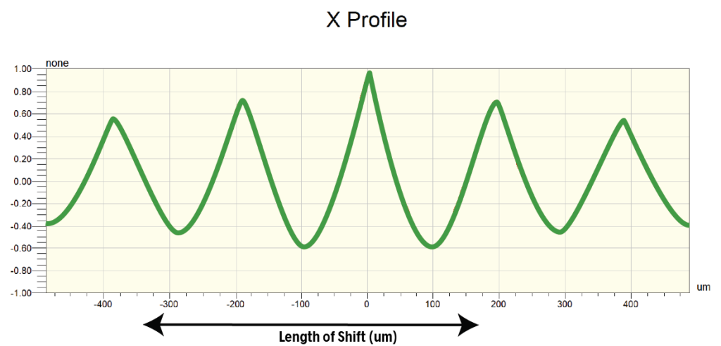
For this turned surface texture, the ACF in the X direction falls from 1 to 0 zero quickly, then becomes negative as the peaks of the shifted surface align with the valleys of the original surface:
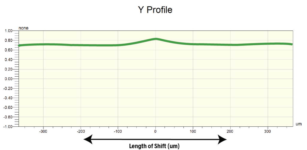
Shifting the duplicate in the Y direction, however, produces very little change, as the texture is very similar along the Y direction. The ACF in the Y direction therefore remains near 1.00.
Note: Autocovariance is a similar parameter, the difference being that it is not normalized to a range of -1.00 to 1.00.
Applying ACF to Solve an Engine Noise Problem
This example shows how ACF can be used to spot periodicity in surface texture that could lead to noise, excessive wear or poor performance.
In this example, an engine noise problem was traced to a particular steel shaft. Surface texture was suspected, and thus the average roughness of a sampling of “quiet” and “noisy” shafts was analyzed. However, the average roughness was well within specification for all of the parts, noisy and quiet.
The engineers decided to have a look at the autocorrelation function to see whether there was any apparent periodicity in the data. A stitched 3D optical profiler image of a “quiet” shaft appeared as follows:

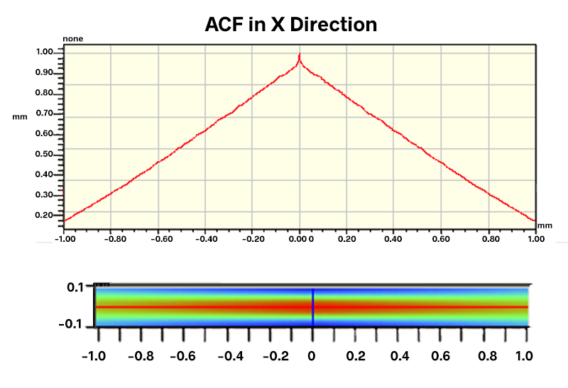
The ACF for this section of the shaft indicates a smooth surface without periodic features:
Optical profiler measurements of the “noisy” shafts, however, revealed what appeared to be a periodic pattern around the shaft:

Indeed, analysis of the ACF brought the periodic pattern into sharp focus:
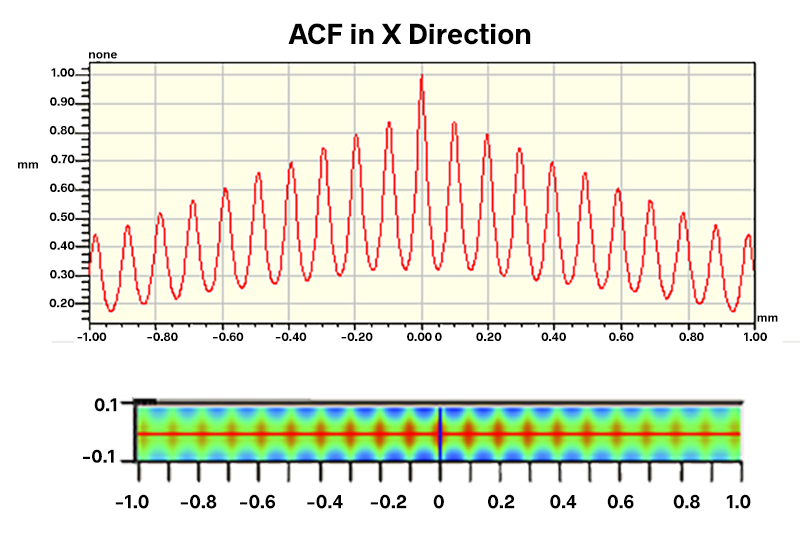
Knowing the period of the texture and its strong directionality, engineers suspected an issue with a grinding operation, possibly a poorly dressed wheel. Specifications were built into the process based on these 3D parameters in order to control the grinding operation.
