Wear between two surfaces in contact can take the form of mechanisms such as ploughing, abrasion, adhesion, fatigue, etc.
The initial phase of a component’s life will involve some period of “running in,” during which peak material will be worn away or deformed, and valleys will be filled in with debris. Run-in is inevitable and, to an extent, can be beneficial. A cylinder ring in contact with a cylinder wall, for example, will conform in a way unique to that pair of components to create an optimal seal.
The goal for engineers is not necessarily to minimize run-in wear but to optimize this important part of the component’s life cycle. To do so, one must first understand what the surface needs to look like for the majority of its life, and then backtrack to estimate how the surface must look just after manufacturing in order to achieve that desired long-term surface after a period of wear. It’s no easy feat, but there are some tools that can help.
A Worn Surface Appears “Filtered”
Just a quick reminder that surface texture is best described as a composite of spatial wavelengths. Shorter wavelength (high spatial frequency) texture is the regime of roughness, while longer wavelengths (low spatial frequency) are considered waviness. The longest wavelengths are considered “form,” which describes the essential shape of the component.
When a machined component leaves the factory its surface may have sharp peaks and crisp valleys from well-controlled machining processes. During the initial wear period the peak material (the summits which actually contact the mating surface) is typically deformed plastically. In the image below you can see the impact of various wear mechanisms on the original profile.
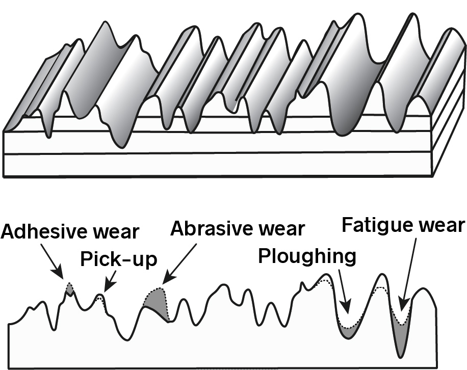
Christiansen, S., De Chiffer, I, Topographic Characterization of Progressive Wear on Deep Drawing Dies, 1997, Tribology Transactions, Vol. 40, 2, 346-352.
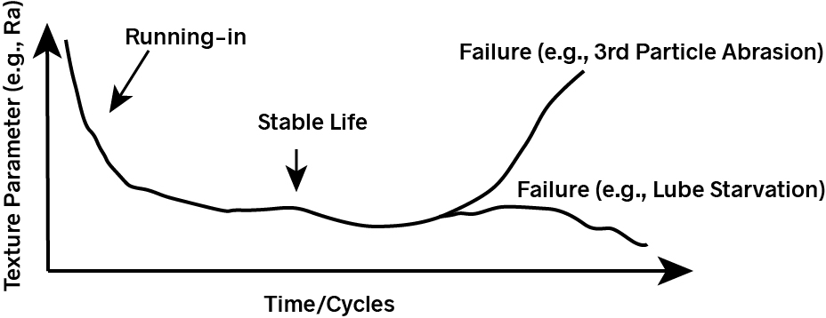
If we were to look at a parameter such as Ra (Average Roughness) we would see that it diminishes during the run-in wear period as peak material is worn and valleys fill in with the debris. At some point the wear rate will slow and the component will enter a period of “stable life,” during which the surface will change very little.
But while average roughness tells us that the surface has changed, it tells us little about how it has changed. If, instead, we look at the wavelength content before and after wear we will see that the short spatial wavelength/ high aspect ratio structures are primarily impacted. Longer wavelength structures become more dominant in relation, as the peak material is worn away. In effect, wear during run-in has the appearance of data to which a low spatial frequency pass filter has been applied.
Using a Filter to Simulate Wear
Knowing this fact, we can make some predictions about how a surface will wear. We can, for example, take a measurement of a surface just after manufacture, then apply a low pass spatial frequency filter to simulate what it may look like after a period of running-in.
Some researchers have done just that, in fact. The example below is based on work by Rosen, Ohlsson and Thomas on the progression of wear of a cylinder bore wall study. Knowing that the summits with the smallest radii deform plastically (crush), while broader summits will compress elastically, they were able to simulate the wear by filtering the original data.
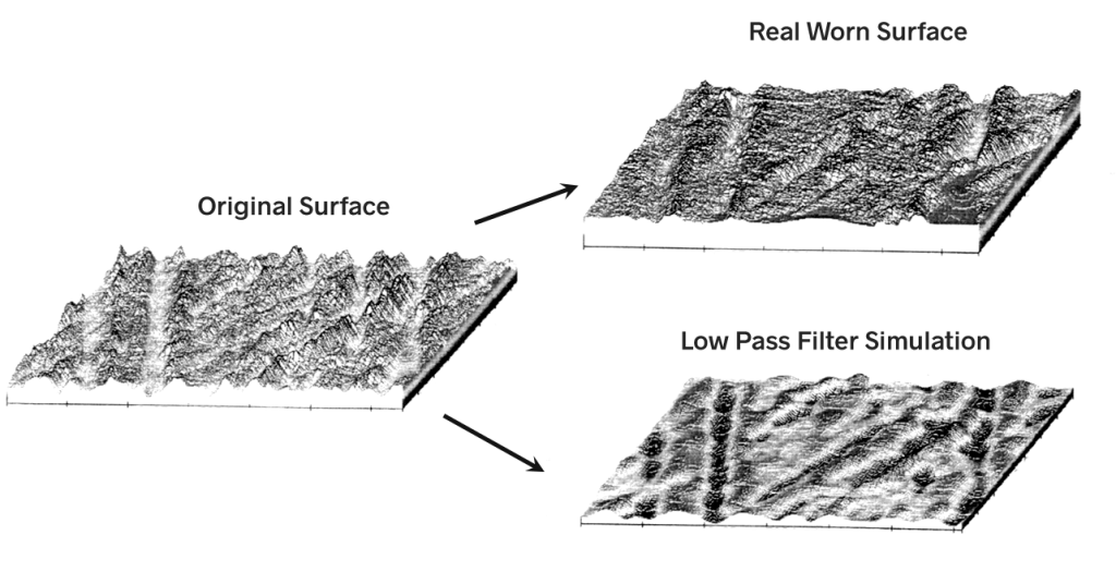
Rosén, B.G, Ohlsson, R., Thomas, T.R., 1995, from Wear of Cylinder Bore Microtopography, Department of Production Engineering, Chalmers University of Technology.
Other surface texture parameters can also be helpful in analyzing and estimating wear. The “bearing ratio” parameters Rpk, Rk and Rvk can help us differentiate the ratio of peaks, valleys and core material, as well as showing how the ratio may change over time. The areal (3D) texture parameters Sds (Summit Density) and Ssc (Summit Curvature) can also help.
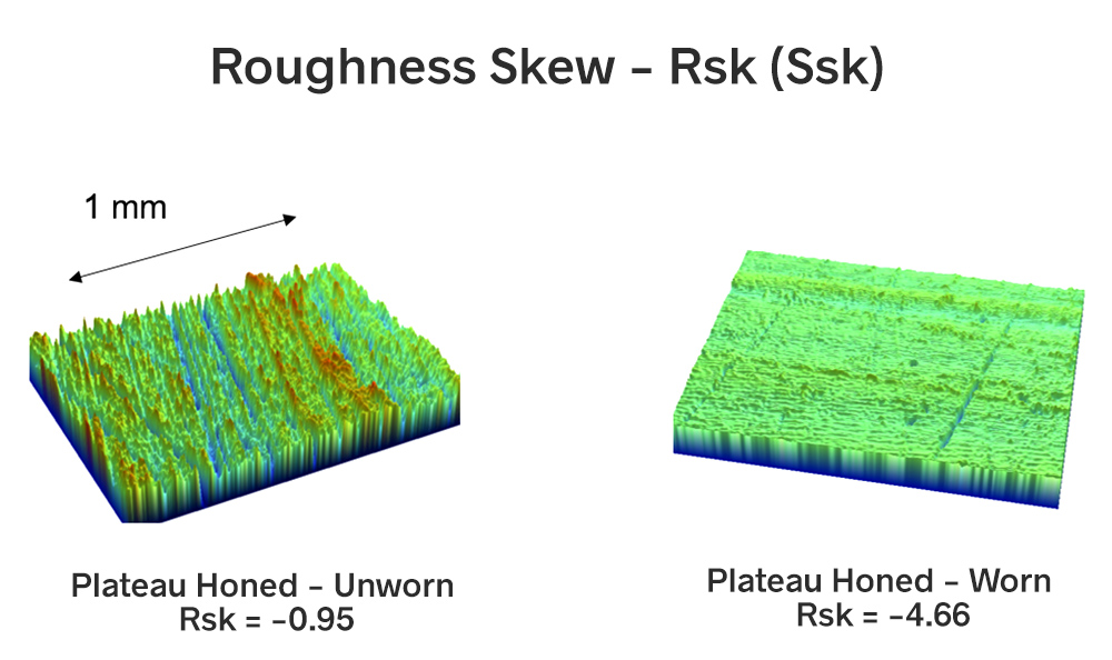
We might also turn to a parameter such as Rsk (Ssk), the Skewness, which is an indicator of the “spikiness” of a surface. Rsk can be a good indicator of how much of a surface will be eroded during initial wear. In this example, the Rsk value dropped from -0.95 to -4.66 during the run-in period as the tall, narrow peaks of material were worn away.
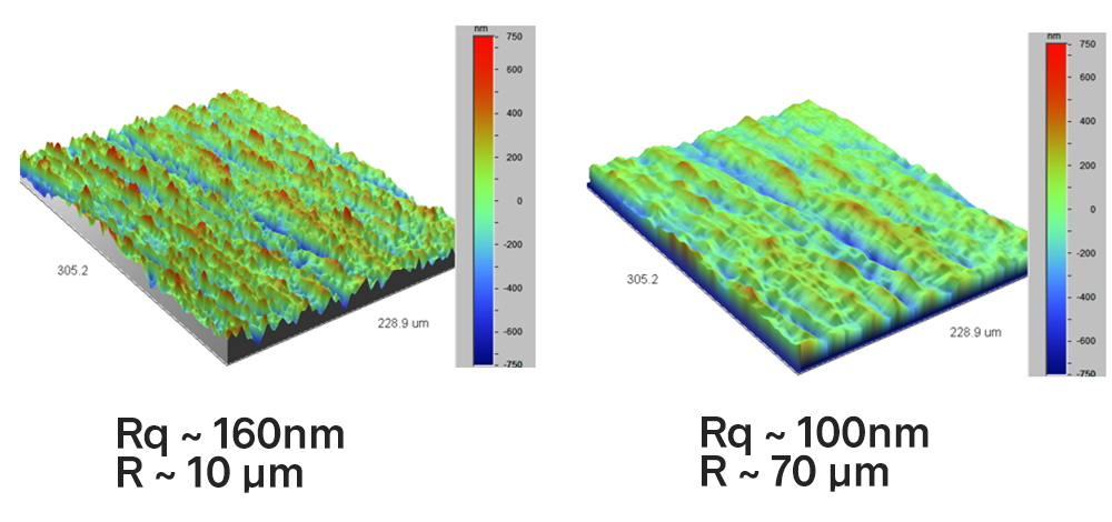
Changes in Rq (Root Mean Square Roughness) and R (Radius of Curvature of the surface summits) can similarly indicate wear. During run-in the Rq in this example drops from 160 nm to 100 nm as peak material is worn. The Radius of Curvature increases from 10 µm to 70 µm as the small-radius summits are worn away, leaving the more durable, larger radius summits. Note that R equals 1/Ssc.
Process to Optimize Run-in
To revisit our goals, again: using surface texture analysis, such as simulating wear with filters, we gain an idea of what a surface should look after manufacturing in order to produce a surface that is optimal for long-term performance after wear-in. The last piece in that puzzle is to consider whether the required run-in period is acceptable. For example, if a car engine takes too long to run in, variability introduced by driver’s habits may make it difficult to estimate the engine’s longevity and meet warranty goals.
There are options, however, to expedite or slow the run-in process, or to alter the amount of material worn away during run-in. One could add a final machining process such as burnishing or ballizing to crush peak material in a controlled fashion. Applying an anti-friction coating may reduce the amount of material that is worn away. Finally, it may be determined that some duration of wear-in should be accomplished at the factory, under controlled conditions, to reach the stable state.
In all cases, being able to measure, and possibly predict, wear on components before and after run-in helps ensure long-term quality of components in contact.
Interested in surface texture parameters that can help with wear measurement?
Read more in the Texture Parameters Glossary.